Relationship Map

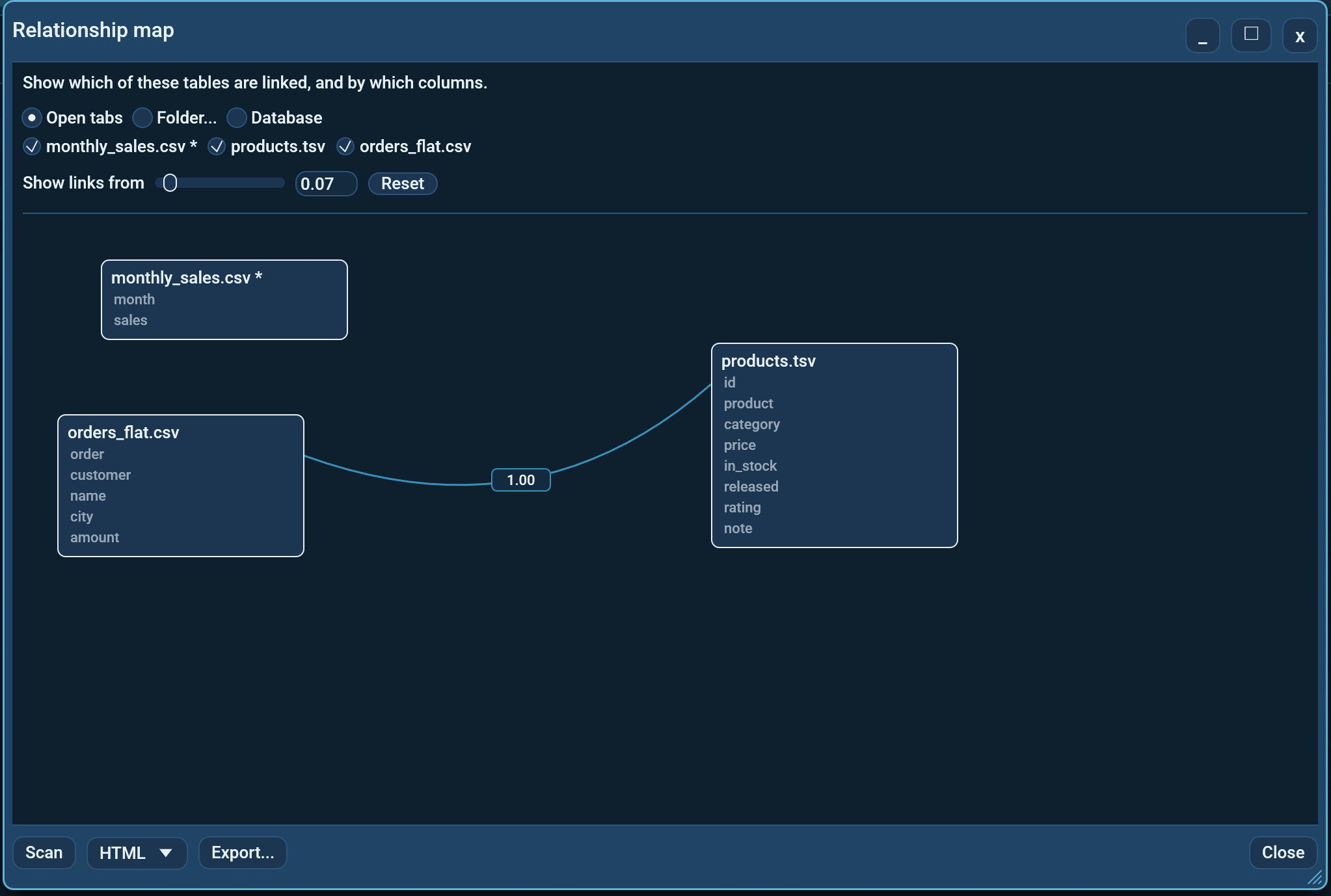
Analyse -> Relationship map... draws how your tables connect: one box per table listing its columns, a line between each pair of columns that relate, and a plain sentence on every line saying how well they match.

It answers the question you have when someone hands you a folder of exports and no diagram.

What decides a line

The same ranking as the Join Key Finder, which is where the arithmetic is set out in full, with a worked example you can check by hand. Column names take no part in it - only values.

The short form. Each column of each table becomes the set of its distinct values, read from a sample of rows, trimmed to text, empty cells skipped. For every pair of columns across two tables:

shared       = how many values appear in BOTH distinct sets
overlap      = shared / the smaller of the two distinct counts
distinctness = distinct values / non-empty values sampled   (each side)

score        = overlap x the LARGER of the two distinctness values

orphans      = distinct values on this side - shared    (counted BOTH ways)

• overlap is 1.00 when every value of the smaller side also exists on the larger side.
• distinctness is how close a column is to having a different value in every row. A primary key is 1.00; a status column with three values across ten thousand rows is 0.0003.
• Taking the larger of the two is deliberate. A foreign key is unique on the parent side and repeats on the child side, so the child's distinctness is low by design; asking whether either side identifies a row is the question that has a yes for every real key.

Multiplying is what stops a status column that happens to overlap perfectly from outranking a real key: its overlap is 1.00, its distinctness is tiny, so its score is tiny. Worth knowing that this is the only thing separating them, since a status pair typically has a perfect overlap and no orphans at all.

A line is drawn when its score reaches the threshold, shown as Show links from under the source options and set to 0.50 by default. Read that as a statement about the two factors together: a pair whose values overlap completely needs the more distinct side to be at least half distinct, and a pair that overlaps only half the time needs a side that is essentially unique.

Move the slider down to see weaker or partial links - a foreign key that only half the rows use will sit well below 0.50 - and up to keep only the strongest. The box beside it takes any value between 0 and 1 typed exactly, with either . or , as the decimal mark; the slider is for sweeping, the box for pinning a number down. It takes effect on the next Scan, not immediately, because the threshold is applied while the values are being compared.

Each line also carries an orphan count: how many distinct values on one side find no partner on the other. That is the number meant to separate two candidates which score identically, and they do exactly when both tables number their rows from 1: with 1,000 orders and 4 customers, orders.id -> customers.id and orders.customer_id -> customers.id both score a perfect 1.00, and only the first leaves 996 orphans.

An orphan count is directional, and the two ways round answer different questions ("customers who never ordered" against "orders pointing at a customer who is gone"). Only one of them can settle a tie, and nothing in the arithmetic knows which of your tables is the child, so both counts are reported on every line: hovering shows one sentence per direction. In the example above the customers side reads 0 for both candidates while the orders side reads 996 and 0, which is the answer. The Join Key Finder page works that example through with real output.

A declared foreign key has no ambiguity to begin with: it already knows which end is the child, and Measure scores it in that direction, so its left-hand count is always child rows pointing at a parent that does not exist.

The orphan count is computed from the same sampled sets the score came from, so the two numbers on one line can never contradict each other.

Boxes that hold more than they show

A box lists the first twelve columns and then a +N row saying how many it left out. That row is a button: click it and the box lists every column, click the -N it turns into and it folds back.

Expanding is not only cosmetic. A line attaches to the row of the column it names, and a column past the twelfth has nowhere to attach while the box is folded, so it lands on the last visible row. Open the box and the line moves to the column it is really about. Dragging the box still works from anywhere, including that row.

Hovering a line reads like a sentence:

98 of 100 values in orders.customer_id exist in customers.id.
2 have no match.

From a live database, no guessing at all

The two sources above read values and infer. A Database source does not have to: somebody already declared the foreign keys, and the server will hand them over for the asking.

Pick Database, choose a saved connection, tick the schemas you care about, and Scan. That reads catalog information only, no table data, so it answers in about as long as any other catalog query no matter how large the tables are. Every line is a declared foreign key and carries its constraint name in the tooltip.

Because nothing was measured, the chips read FK rather than a score. A declaration and a fact are not the same thing:

• Postgres, MySQL, SQL Server and Exasol enforce their foreign keys, so a line from those servers is also true of the rows.
• Redshift, Snowflake, Databricks and BigQuery accept a declaration and enforce nothing. A child value pointing at a parent that does not exist is entirely possible there.

Measure is the answer to that. It reads a sample of rows from each drawn table and fills in the same overlap, score and orphan count the value-based sources carry, so a declared key that nothing honours shows up as orphans. It is a separate button and never automatic, because it is the step that actually reads your data.

The Tables list under the schemas holds every table the scan saw. Tables taking part in a foreign key start ticked; the rest do not, since a grid of boxes with no lines between them is an inventory, not a map. Ticking one redraws immediately, without asking the server again.

ClickHouse has no referential constraints of any kind, so there is nothing to read there; map its tables as files or open tabs instead.

Using it

1. Analyse -> Relationship map...
2. Choose the source: the open tabs you tick, a folder of data files, or a live database.
3. Scan. Reading values takes a moment, so it runs in the background with a Cancel button.
4. Drag the boxes into an arrangement that suits you.
5. Drag a score chip to bend its line. The chip is the curve's handle: the whole connection follows it, so two lines running through the same space can be pulled apart instead of overlapping. A chip you have not touched leaves its line straight.
6. Click a line to open the Join dialog with that pair already filled in.

Exporting the map

Export... at the bottom writes the map as it stands at that moment: the boxes where you dragged them, the lines bent the way you bent them, and the column lists open as far as you opened them. It is not a fresh layout of the same data.

The picker beside the button chooses the format and remembers the choice, so if you always want SVG you set it once (it is stored as rel_map_export_format in settings.toml):

Format	Good for
PDF (default)	Putting in a document, printing. Vector, sharp at any size.
SVG	Editing afterwards in Inkscape or Illustrator, or embedding in a page.
PNG	Pasting into a chat or a slide. Rendered at 2x so it stays crisp.
HTML	Sending to someone who does not have Octa, while keeping it interactive.

Nothing is a screenshot. All four go through one hand-emitted SVG, so the export does not depend on your window size, your zoom or your screen's DPI, and it uses the colours of the theme you are running.

The HTML export stays interactive

The HTML file is one self-contained page: no libraries, no fonts and no images are fetched, so it opens from a USB stick or an email attachment, and it works offline.

The drawing fills the whole window, so a box can be dragged anywhere on screen without being cut off or becoming ungrabbable.

In the browser you can:

• pan by dragging the background, zoom with the wheel (about the pointer, so what is under the cursor stays put), and Reset view;
• drag the boxes, with every connected line re-routing live, including the bend you gave it;
• hover a line for the same sentence Octa shows.

What it does not carry over is bending a line, clicking through to the Join dialog, and Measure. Those need Octa.

From the command line

octa --relationships ./exports
octa --relationships ./exports --recursive

Prints the ranked pairs best first, with the same numbers the map draws and both orphan counts:

$ octa --relationships ./example
left_table     left_column  right_table  right_column  score  overlap  left_orphans  left_values  right_orphans  right_values
customers.csv  id           orders.csv   cust_id       1      1        1             4            0              3
customers.csv  status       orders.csv   status        0.5    1        0             2            0              2

Always exits 0: this is a report, not a gate. Unreadable files are named on stderr.

--relationships scans a folder. For the declared keys of a live database, use the Database source above or the db_relationships tool, which the Assistant can call as well.

Limits

• Sampled, 10,000 rows per table. Strong evidence, not a certified foreign key.
• Single columns only. A composite key is not suggested; use --unique-columns for that question.
• Values are compared as trimmed text, so 1 and 1.0 are different.
• A folder scan reads at most 30 files, and a database scan at most 30 tables; both say when they stopped.
• A declared key whose other end is not drawn is counted and reported, not drawn as a line into nowhere.
• Orphan counts are reported in both directions, but nothing labels which table is the child; you read that off the two numbers. A declared key measured from a database is always counted child to parent.
• Clicking a line prefills the Join dialog only for open tabs; a folder scan draws the map and leaves the joining to you.
• Expanding a box is remembered for as long as the map is; a new Scan folds every box back, because the tables may be different ones.